Principal component analysis (PCA) and visualization using Python (Detailed guide with example)

Page content

• What is Principal component analysis (PCA)?
• Perform PCA in Python
  • load dataset
  • Standardization
  • Perform PCA using scikit-learn
  • Principal component (PC) retention
  • PCA loadings plots
  • PCA biplot
  • PCA biplot
• PCA interpretation
• PCA interpretation
• Principal component analysis (PCA) with a target variable
• PCA from scratch
  • Calculate mean adjusted matrix
  • Calculate the covariance matrix
  • Eigendecomposition of the covariance matrix

What is Principal component analysis (PCA)?

• PCA is a classical multivariate (unsupervised machine learning) non-parametric dimensionality reduction method that used to interpret the variation in high-dimensional interrelated dataset (dataset with a large number of variables)
• PCA reduces the high-dimensional interrelated data to low-dimension by linearly transforming the old variable into a new set of uncorrelated variables called principal component (PC) while retaining the most possible variation.
• The first component has the largest variance followed by the second component and so on. The first few components retain most of the variation, which is easy to visualize and summarise the feature of original high-dimensional datasets in low-dimensional space. PCA helps to assess which original samples are similar and different from each other.
• PCA preserves the global data structure by forming well-separated clusters but can fail to preserve the similarities within the clusters.
• PCA works better in revealing linear patterns in high-dimensional data but has limitations with the nonlinear dataset. The t-SNE can be used for dimensionality reduction for nonlinear datasets.
• For example, when datasets contain 10 variables (10D), it is arduous to visualize them at the same time (you may have to do 45 pairwise comparisons to interpret dataset effectively). PCA transforms them into a new set of variables (PCs) with top PCs having the highest variation. PCs are ordered which means that the first few PCs (generally first 3 PCs but can be more) contribute most of the variance present in the the original high-dimensional dataset. These top first 2 or 3 PCs can be plotted easily and summarize and the features of all original 10 variables.
• PCA is a useful method in the Bioinformatics field, where high-throughput sequencing experiments (e.g. RNA-seq, GWAS) often leads to the generation of high-dimensional datasets (a few hundred to thousands of samples). For example, in RNA-seq experiments PCA helps to understand the gene expression patterns and biological variation in a high-dimensional RNA-seq datasets.

Perform PCA in Python

• we will use sklearn, seaborn, and bioinfokit (v2.0.2 or later) packages for PCA and visualization (check how to install Python packages)
• Download dataset for PCA (a subset of gene expression data associated with different conditions of fungal stress in cotton which is published in Bedre et al., 2015)

Note: If you have your own dataset, you should import it as pandas dataframe. Learn how to import data using pandas

load dataset

from sklearn.decomposition import PCA
from sklearn.preprocessing import StandardScaler
from bioinfokit.analys import get_data
import numpy as np
import pandas as pd
# load dataset as pandas dataframe
df = get_data('gexp').data
df.head(2)
# output
         A        B        C        D        E         F
0  4.50570  3.26036 -1.24940  8.89807  8.05955 -0.842803
1  3.50856  1.66079 -1.85668 -2.57336 -1.37370  1.196000
# variables A to F denotes multiple conditions associated with fungal stress
# Read full paper https://journals.plos.org/plosone/article?id=10.1371/journal.pone.0138025

sample size recommendations for PCA

• As PCA is based on the correlation of the variables, it usually requires a large sample size for the reliable output. The sample size can be given as the absolute numbers or as subjects to variable ratios.
• The minimum absolute sample size of 100 or at least 10 or 5 times to the number of variables is recommended for PCA. On other hand, Comrey and Lee’s (1992) have a provided sample size scale and suggested the sample size of 300 is good and over 1000 is excellent.
• As a rule of thumb, the minimum sample size of 100 (or more is better) would be sufficient for PCA analysis.

Standardization

• Standardization dataset with (mean=0, variance=1) scale is necessary as it removes the biases in the original variables. For example, when the data for each variable is collected on different units.
• The standardized variables will be unitless and have a similar variance.
• Standardization is an advisable method for data transformation when the variables in the original dataset have been measured on a significantly different scale.
• At some cases, the dataset needs not to be standardized as the original variation in the dataset is important (Gewers et al., 2018)

# this is an optional step
df_st =  StandardScaler().fit_transform(df)  
pd.DataFrame(df_st, columns=df.columns).head(2)
# output
          A         B         C         D         E         F
0  0.619654  0.448280 -0.240867  2.457058  2.304732 -0.331489
1  0.342286 -0.041499 -0.428652 -1.214732 -0.877151  0.474930

Perform PCA using scikit-learn

pca_out = PCA().fit(df_st)

# get the component variance
# Proportion of Variance (from PC1 to PC6)
pca_out.explained_variance_ratio_
# output
array([0.2978742 , 0.27481252, 0.23181442, 0.19291638, 0.00144353,
       0.00113895])

# Cumulative proportion of variance (from PC1 to PC6)   
np.cumsum(pca_out.explained_variance_ratio_)
# output
array([0.2978742 , 0.57268672, 0.80450114, 0.99741752, 0.99886105,
       1.        ])
       
# component loadings or weights (correlation coefficient between original variables and the component) 
# component loadings represents the elements of the eigenvector
# the squared loadings within the PCs always sums to 1
loadings = pca_out.components_
num_pc = pca_out.n_features_
pc_list = ["PC"+str(i) for i in list(range(1, num_pc+1))]
loadings_df = pd.DataFrame.from_dict(dict(zip(pc_list, loadings)))
loadings_df['variable'] = df.columns.values
loadings_df = loadings_df.set_index('variable')
loadings_df
# output
               PC1       PC2       PC3       PC4       PC5       PC6
variable
A        -0.510898  0.452234  0.227356 -0.323464  0.614881  0.008372
B        -0.085908  0.401197  0.708556  0.132788 -0.558448 -0.010616
C         0.477477 -0.100994  0.462437  0.487951  0.556605  0.007893
D         0.370318  0.611485 -0.308295  0.054973 -0.007642  0.625159
E         0.568491  0.300118 -0.011775 -0.484115  0.009382 -0.593425
F         0.208090 -0.400426  0.370440 -0.634234 -0.010111  0.506732

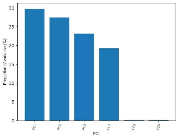
# positive and negative values in component loadings reflects the positive and negative 
# correlation of the variables with the PCs. Except A and B, all other variables have 
# positive projection on first PC.

# get correlation matrix plot for loadings
import seaborn as sns
import matplotlib.pyplot as plt
ax = sns.heatmap(loadings_df, annot=True, cmap='Spectral')
plt.show()

Generated correlation matrix plot for loadings,

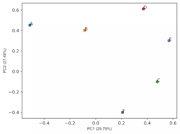
Principal component (PC) retention

• As the number of PCs is equal to the number of original variables, We should keep only the PCs which explain the most variance (70-95%) to make the interpretation easier. More the PCs you include that explains most variation in the original data, better will be the PCA model. This is highly subjective and based on the user interpretation (Cangelosi et al., 2007).
• The eigenvalues (variance explained by each PC) for PCs can help to retain the number of PCs. Generally, PCs with eigenvalues > 1 contributes greater variance and should be retained for further analysis.
• Scree plot (for elbow test) is another graphical technique useful in PCs retention. We should keep the PCs where there is a sharp change in the slope of the line connecting adjacent PCs.

# get eigenvalues (variance explained by each PC)  
pca_out.explained_variance_
# output
array([1.78994905, 1.65136965, 1.39299071, 1.15924943, 0.0086743 ,
       0.00684401])
# get scree plot (for scree or elbow test)
from bioinfokit.visuz import cluster
cluster.screeplot(obj=[pc_list, pca_out.explained_variance_ratio_])
# Scree plot will be saved in the same directory with name screeplot.png

Generated Scree plot,

PCA loadings plots

# get PCA loadings plots (2D and 3D)
# 2D
cluster.pcaplot(x=loadings[0], y=loadings[1], labels=df.columns.values, 
    var1=round(pca_out.explained_variance_ratio_[0]*100, 2),
    var2=round(pca_out.explained_variance_ratio_[1]*100, 2))

# 3D
cluster.pcaplot(x=loadings[0], y=loadings[1], z=loadings[2],  labels=df.columns.values, 
    var1=round(pca_out.explained_variance_ratio_[0]*100, 2), var2=round(pca_out.explained_variance_ratio_[1]*100, 2), 
    var3=round(pca_out.explained_variance_ratio_[2]*100, 2))

Generated 2D PCA loadings plot (2 PCs) plot,

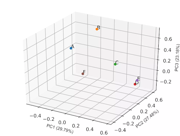
Generated 3D PCA loadings plot (3 PCs) plot,

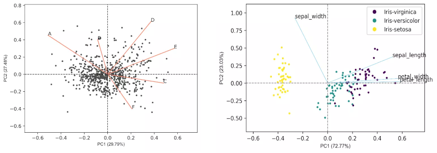
PCA biplot

• In biplot, the PC loadings and scores are plotted in a single figure
• biplots are useful to visualize the relationships between variables and observations

# get PC scores
pca_scores = PCA().fit_transform(df_st)

# get 2D biplot
cluster.biplot(cscore=pca_scores, loadings=loadings, labels=df.columns.values, var1=round(pca_out.explained_variance_ratio_[0]*100, 2),
    var2=round(pca_out.explained_variance_ratio_[1]*100, 2))
    
# get 3D biplot
cluster.biplot(cscore=pca_scores, loadings=loadings, labels=df.columns.values, 
    var1=round(pca_out.explained_variance_ratio_[0]*100, 2), var2=round(pca_out.explained_variance_ratio_[1]*100, 2), 
    var3=round(pca_out.explained_variance_ratio_[2]*100, 2))

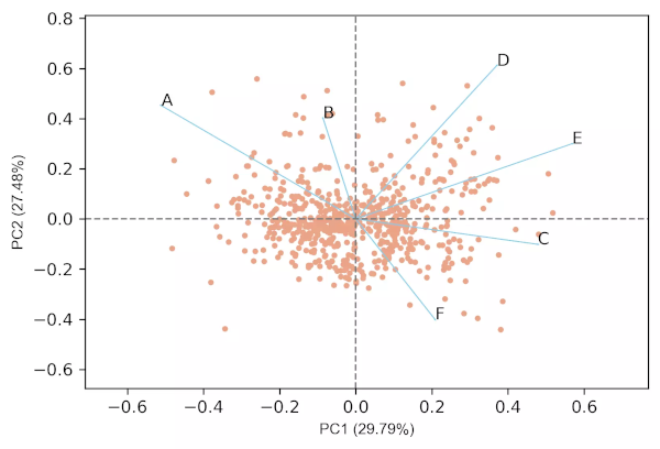
Generated 2D biplot,

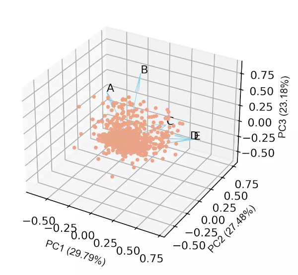
Generated 3D biplot,

In addition to these features, we can also control the label fontsize, figure size, resolution, figure format, and other many parameters for scree plot, loadings plot and biplot.

Check detailed usage

PCA interpretation

• The first three PCs (3D) contribute ~81% of the total variation in the dataset and have eigenvalues > 1, and thus provides a good approximation of the variation present in the original 6D dataset (see the cumulative proportion of variance and scree plot). The cut-off of cumulative 70% variation is common to retain the PCs for analysis (Jolliffe et al., 2016). Even though the first four PCs contribute ~99% and have eigenvalues > 1, it will be difficult to visualize them at once and needs to perform pairwise visualization.
• From the biplot and loadings plot, we can see the variables D and E are highly associated and forms cluster (gene expression response in D and E conditions are highly similar). Similarly, A and B are highly associated and forms another cluster (gene expression response in A and B conditions are highly similar but different from other clusters). If the variables are highly associated, the angle between the variable vectors should be as small as possible in the biplot.
• The length of PCs in biplot refers to the amount of variance contributed by the PCs. The longer the length of PC, the higher the variance contributed and well represented in space.

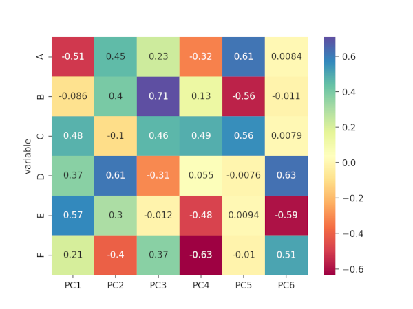
Principal component analysis (PCA) with a target variable

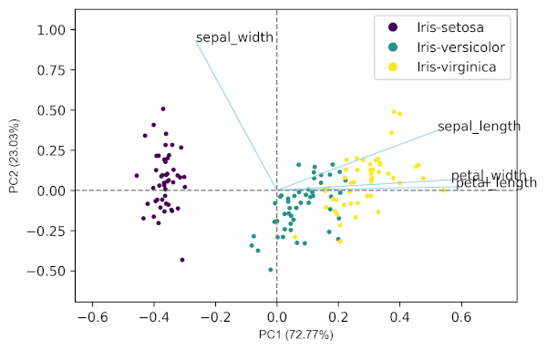
• We have covered the PCA with a dataset that does not have a target variable. Now, we will perform the PCA on the iris plant dataset, which has a target variable.

from sklearn.decomposition import PCA
from sklearn.preprocessing import StandardScaler
from bioinfokit.analys import get_data
from bioinfokit.visuz import cluster

# load iris dataset
df = get_data('iris').data
df.head(2)
# output 
# class (type of iris plant) is target variable
   sepal_length  sepal_width  petal_length  petal_width        class
0           5.1          3.5           1.4          0.2  Iris-setosa
1           4.9          3.0           1.4          0.2  Iris-setosa

X = df.iloc[:,0:4]
target = df['class'].to_numpy()
X.head(2)
   sepal_length  sepal_width  petal_length  petal_width
0           5.1          3.5           1.4          0.2
1           4.9          3.0           1.4          0.2

X_st =  StandardScaler().fit_transform(X)
pca_out = PCA().fit(X_st)

# component loadings
loadings = pca_out.components_
loadings
array([[ 0.52237162, -0.26335492,  0.58125401,  0.56561105],
       [ 0.37231836,  0.92555649,  0.02109478,  0.06541577],
       [-0.72101681,  0.24203288,  0.14089226,  0.6338014 ],
       [-0.26199559,  0.12413481,  0.80115427, -0.52354627]])

# get eigenvalues (variance explained by each PC)  
pca_out.explained_variance_
array([2.93035378, 0.92740362, 0.14834223, 0.02074601])

# get biplot
pca_scores = PCA().fit_transform(X_st)
cluster.biplot(cscore=pca_scores, loadings=loadings, labels=X.columns.values, var1=round(pca_out.explained_variance_ratio_[0]*100, 2),
    var2=round(pca_out.explained_variance_ratio_[1]*100, 2), colorlist=target)

Generated biplot,

PCA from scratch

• Computing the PCA from scratch involves various steps, including standardization of the input dataset (optional step), calculating mean adjusted matrix, covariance matrix, and calculating eigenvectors and eigenvalues.

Calculate mean adjusted matrix

from bioinfokit.analys import get_data
from sklearn.preprocessing import StandardScaler
import pandas as pd
# load iris dataset
df = get_data('iris').data
df.head(2)
   sepal_length  sepal_width  petal_length  petal_width        class
0           5.1          3.5           1.4          0.2  Iris-setosa
1           4.9          3.0           1.4          0.2  Iris-setosa
# the iris dataset has 150 samples (n) and 4 variables (p), i.e., nxp matrix

X = df.iloc[:,0:4]  # p variables
target = df['class'].to_numpy()  # target variable

# standardize the dataset (this is an optional step)
# I am using this step to get consistent output as per the PCA method used above
X_st =  StandardScaler().fit_transform(X)
X_st = pd.DataFrame(X_st)
X_st.columns = X.columns

# create mean adjusted matrix (subtract each column mean by its value)
X_adjusted = X_st - X_st.mean()
X_adjusted.head(2)
   sepal_length  sepal_width  petal_length  petal_width
0     -0.900681     1.032057     -1.341272    -1.312977
1     -1.143017    -0.124958     -1.341272    -1.312977

Calculate the covariance matrix

X_adjusted.cov()
              sepal_length  sepal_width  petal_length  petal_width
sepal_length      1.006711    -0.110103      0.877605     0.823443
sepal_width      -0.110103     1.006711     -0.423338    -0.358937
petal_length      0.877605    -0.423338      1.006711     0.969219
petal_width       0.823443    -0.358937      0.969219     1.006711

Eigendecomposition of the covariance matrix

• Eigendecomposition of covariance matrix yields eigenvectors (PCs) and eigenvalues (variance of PCs). The elements of eigenvectors are known as loadings. This step involves linear algebra and can be performed using NumPy linalg.eig function. This is a very important step in PCA.

from numpy.linalg import eig
eigenvalues, eigenvectors = eig(X_adjusted.cov())
eigenvalues
array([2.93035378, 0.92740362, 0.14834223, 0.02074601])
# we are interested in highest eigenvalues as it explains most of the variance
# this helps to reduce the dimensions

eigenvectors
array([[ 0.52237162, -0.37231836, -0.72101681,  0.26199559],
       [-0.26335492, -0.92555649,  0.24203288, -0.12413481],
       [ 0.58125401, -0.02109478,  0.14089226, -0.80115427],
       [ 0.56561105, -0.06541577,  0.6338014 ,  0.52354627]])

# column eigenvectors[:,i] is the eigenvectors of eigenvalues eigenvalues[i]

Enhance your skills with courses on Machine Learning

• Machine Learning Specialization
• Principal Component Analysis with NumPy
• Mathematics for Machine Learning: PCA
• Dimensionality Reduction in Python
• Python for Genomic Data Science
• Bioinformatics Specialization
• Command Line Tools for Genomic Data Science

Related reading

• k-means clustering in Python [with example]
• Support Vector Machine (SVM) basics and implementation in Python
• Logistic regression in Python (feature selection, model fitting, and prediction)

References

• Pedregosa F, Varoquaux G, Gramfort A, Michel V, Thirion B, Grisel O, Blondel M, Prettenhofer P, Weiss R, Dubourg V, Vanderplas J. Scikit-learn: Machine learning in Python. the Journal of machine Learning research. 2011 Nov 1;12:2825-30.
• Abdi H, Williams LJ. Principal component analysis. Wiley interdisciplinary reviews: computational statistics. 2010 Jul;2(4):433-59.
• Jolliffe IT, Cadima J. Principal component analysis: a review and recent developments. Philosophical Transactions of the Royal Society A: Mathematical, Physical and Engineering Sciences. 2016 Apr 13;374(2065):20150202.
• Gewers FL, Ferreira GR, de Arruda HF, Silva FN, Comin CH, Amancio DR, Costa LD. Principal component analysis: A natural approach to data exploration. arXiv preprint arXiv:1804.02502. 2018 Apr 7.
• Bedre R, Rajasekaran K, Mangu VR, Timm LE, Bhatnagar D, Baisakh N. Genome-wide transcriptome analysis of cotton (Gossypium hirsutum L.) identifies candidate gene signatures in response to aflatoxin producing fungus Aspergillus flavus. PLoS One. 2015;10(9).
• Kirkwood RN, Brandon SC, de Souza Moreira B, Deluzio KJ. Searching for stability as we age: the PCA-Biplot approach. International Journal of Statistics in Medical Research. 2013 Oct 1;2(4):255.
• Cangelosi R, Goriely A. Component retention in principal component analysis with application to cDNA microarray data. Biology direct. 2007 Dec 1;2(1):2.
• Vallejos CA. Exploring a world of a thousand dimensions. Nature Biotechnology. 2019 Dec;37(12):1423-4.
• Budaev SV. Using principal components and factor analysis in animal behaviour research: caveats and guidelines. Ethology. 2010 May;116(5):472-80.
• Fisher RA. The use of multiple measurements in taxonomic problems. Annals of eugenics. 1936 Sep;7(2):179-88.

This work is licensed under a Creative Commons Attribution 4.0 International License

Some of the links on this page may be affiliate links, which means we may get an affiliate commission on a valid purchase. The retailer will pay the commission at no additional cost to you.