Multiple linear regression (MLR)

Multiple Linear Regression (MLR)
- Multiple Linear Regression (MLR), also called as Multiple Regression, models the linear relationships of one continuous dependent variable by two or more continuous or categorical independent variables. If the dependent variable is measured on an ordinal scale (e.g. Likert-type scale for severity of disease), it is better to use ordinal logistic regression (ordinal regression).
- In contrast to simple linear regression, the MLR model is useful when there are multiple independent variables, as it estimates an individual slope of the regression line for each independent variable.
- If we have n independent variables (
X), the MLR model for predicting the dependent variable (y) can be represented as,
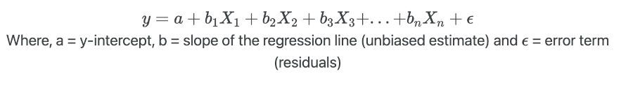
- MLR makes similar assumptions as simple linear regression. In addition, there should be no multicollinearity among the independent variables.
Note: Dependent variable also called a response, outcome, regressand, criterion, or endogenous variable. Independent variable also called explanatory, [covariates](what-is-covariate.html), predictor, regressor, or exogenous variable.
Perform Multiple Linear Regression (MLR) in Python
- For performing the MLR, we will use the plant species richness data to study the influence of different physiographic factors on the native plant richness of islands. The data is collected from 22 different coastal islands (McMaster 2005).
- The dataset contains native plant richness as dependent variable (
y) and area, latitude, and distance from mainlands as independent variables (X). - We will use statsmodels and
bioinfokit v1.0.8or later for performing MLR in Python (check how to install Python packages)
Note: If you have your own dataset, you should import it as a pandas dataframe. Learn how to import data using pandas
Let’s perform MLR in Python
import pandas as pd
import numpy as np
import statsmodels.api as sm
from statsmodels.tools.eval_measures import rmse
from bioinfokit.analys import get_data, stat
from statsmodels.stats.outliers_influence import variance_inflation_factor

# load data
df = get_data('plant_richness').data
df.head(2)
# output
   ntv_rich      area  latitude  dist_mainland
0  1.897627  1.602060     42.99           10.0
1  1.633468  0.477121     41.25            0.3

X = df[['area', 'latitude', 'dist_mainland']]   # independent variables
y = df['ntv_rich']   # dependent variables

# to get intercept -- this is optional
X = sm.add_constant(X)

# fit the regression model
reg = sm.OLS(y, X).fit()
reg.summary()
# output
                            OLS Regression Results
==============================================================================
Dep. Variable:               ntv_rich   R-squared:                       0.915
Model:                            OLS   Adj. R-squared:                  0.901
Method:                 Least Squares   F-statistic:                     64.98
Date:                Sat, 30 Jan 2021   Prob (F-statistic):           7.47e-10
Time:                        00:12:26   Log-Likelihood:                 11.874
No. Observations:                  22   AIC:                            -15.75
Df Residuals:                      18   BIC:                            -11.38
Df Model:                           3
Covariance Type:            nonrobust
=================================================================================
                    coef    std err          t      P>|t|      [0.025      0.975]
---------------------------------------------------------------------------------
const             5.1045      0.981      5.201      0.000       3.043       7.166
area              0.3497      0.027     12.828      0.000       0.292       0.407
latitude         -0.0863      0.023     -3.777      0.001      -0.134      -0.038
dist_mainland    -0.0047      0.003     -1.732      0.100      -0.010       0.001
==============================================================================
Omnibus:                        2.723   Durbin-Watson:                   1.651
Prob(Omnibus):                  0.256   Jarque-Bera (JB):                1.253
Skew:                           0.130   Prob(JB):                        0.534
Kurtosis:                       1.860   Cond. No.                     1.36e+03
==============================================================================

# regression metrics
res= stat()
res.reg_metric(y=np.array(y), yhat=np.array(reg.predict(X)), resid=np.array(reg.resid))
res.reg_metric_df

                                 Metrics   Value
0          Root Mean Square Error (RMSE)  0.1410
1               Mean Squared Error (MSE)  0.0199
2              Mean Absolute Error (MAE)  0.1227
3  Mean Absolute Percentage Error (MAPE)  0.0625

# Variance Inflation Factor (VIF)
# make sure you have added intercept (constant) in X using add_constant(X)
pd.DataFrame({'variables':X.columns[1:], 'VIF':[variance_inflation_factor(X.values, i+1) for i in range(len(X.columns[1:]))]})
# output
       variables       VIF
0           area  1.035192
1       latitude  1.023562
2  dist_mainland  1.026738
Jupyter python notebook: ![]()
Perform Multiple Linear Regression (MLR) in R
Jupyter R notebook: ![]()
Multiple Linear Regression (MLR) interpretation
Regression line
- The regression line with equation [
y = 5.1045 + (0.3497*area) + (-0.0863*latitude) + (-0.0047*dist_mainland)], is helpful to predict the value of the dependent variable (y) from the given value of the independent variables (X). - Regression can be useful in predicting the
yof any value within the range ofX. It also predictsyfromXoutside the given range, but such extrapolation may not be useful.
Root Mean Square Error (RMSE), Mean squared error (MSE), Mean absolute error (MAE), and Mean absolute percent error (MAPE)
- RMSE (0.14) represents the standard deviation of the residuals. It gives an estimate of the spread of observed data points across the predicted regression line. The lower the RMSE, the better is the regression model.
- Mean squared error (MSE) is the mean of the square of residuals. RMSE is a squared root of the MSE.
- Mean absolute error (MAE) represents the mean of absolute differences between actual and predicted values.
- Mean absolute percent error (MAPE) represents the mean of absolute percent differences between actual and predicted values.
Regression coefficients (slope) and constant (y-intercept)
- The regression coefficients or slope (0.34, -0.08, and -0.0047) represent the change in the
yper unit change in theXvariable after adjusting for the simultaneous linear change. It means the valueyincreases by 0.34 (slope forarea) with each unit increase inareaafter adjusting for the simultaneous linear change inlatitudeanddist_mainland. - Similarly, the value
ydecreases by -0.08 with each unit increase inlatitudeafter adjusting for the simultaneous linear change inareaanddist_mainland.Note: There is common practice to interpret the regression coefficients as a change in `y` when other `X` variables are remain constant. This may not be right. Read the full paper from Dr. David C Hoaglin for more details.
- The regression coefficients should be interpreted confidently only if they are statistically significant (p < 0.05).
- The y-intercept (5.10) represents the value of y when all X variables have a value of 0.
- y-intercept should be interpreted cautiously as sometimes the value
Xdoes not make any sense (e.g. speed of car or height of the person). In such cases, the values within the range of X should be considered to interpret the y-intercept. - The p values associated with
areaandlatitudeare significant (p < 0.05). It suggests thatareaandlatitudesignificantly influence the native plant richness.
ANOVA
- In regression, the ANOVA tests the null hypothesis that there is no relationship between the independent variable (
X) and dependent (y) variable i.e. it tests the null hypothesis that regression coefficients equal to zero (b1= b2=…=bn=0). - From ANOVA F test, the p value is significant (<0.05),
which suggests that there is a significant relationship between
Xandy. The independent variables (X) can reliably predict the dependent (y) variable.
Coefficient of determination (R-Squared and adjusted R-Squared)
- The coefficient of determination (R-Squared) is 0.91 (~91%), which suggests that ~91% of the variance in
ycan be explained by X variables. - In MLR, adjusted R-Squared (corrected for sample size and regression coefficients) is more appropriate than
R-Squared as an increasing number of
Xvariables also increases R-Squared. Adjusted R-Squared is always lower than the R-Squared. - Generally, high R-Squared or adjusted R-Squared represents better model, but it is not always true and should be cautiously used for model evaluation based on subject area.
- There is no good cut-off value of R-Squared for good model selection. R-Squared should be evaluated based on field data type, data transformations, or based on subject area decisions. For example, for the nonstationary time series dependent variable, the higher R-Squared (close to 1) may not be good.
Multicollinearity and Variance inflation factor (VIF)
- Multicollinearity (the significant correlation among the
Xvariables) is often a problem. Multicollinearity results in an inflation of variance and, changes in the signs and confidence intervals of regression coefficients (Ryan, 2008). - Therefore, it is necessary to detect and eliminate multicollinearity. Multicollinearity can be detected using correlation analysis or Variance inflation factor (VIF).
- Generally, VIF > 5 or > 10 suggests multicollinearity. But this is not a universal agreement and VIF < 5 could also suggest the multicollinearity. .
- VIF < 2 is a good indicator of the absence of strong multicollinearity and VIF = 1 indicates a complete absence of
multicollinearity. In the above results, the VIF for all the
Xvariables < 2 and suggests there is no strong relationship between the X variables. - A correlation coefficient > 0.5 among the X variables can be used to detect the multicollinearity (Vatcheva et al., 2016).
- To remove the multicollinearity you can either take more measurements or remove the variables causing multicollinearity or perform the ridge regression (Ryan, 2008).
Check Multiple Linear Regression (MLR) Assumptions
Residuals vs fitted (y_hat) plot: This plot used to check for linearity, variances and outliers in the regression data
# get residuals and standardized residuals
from bioinfokit.visuz import stat
df[['yhat']]=pd.DataFrame(reg.predict(X))
df['res']=pd.DataFrame(reg.resid)
df['std_res']=reg.get_influence().resid_studentized_internal
df.head(2)
   ntv_rich      area  latitude  dist_mainland      yhat      res   std_res
0  1.897627  1.602060     42.99           10.0  1.906057 -0.00843 -0.056140
1  1.633468  0.477121     41.25            0.3  1.708459 -0.07499 -0.555013

# create fitted (y_hat) vs residuals plot
stat.reg_resid_plot(df=df, yhat='yhat', resid='res', stdresid='std_res')
# plot will be saved in same dir (resid_plot.png and std_resid_plot.png)
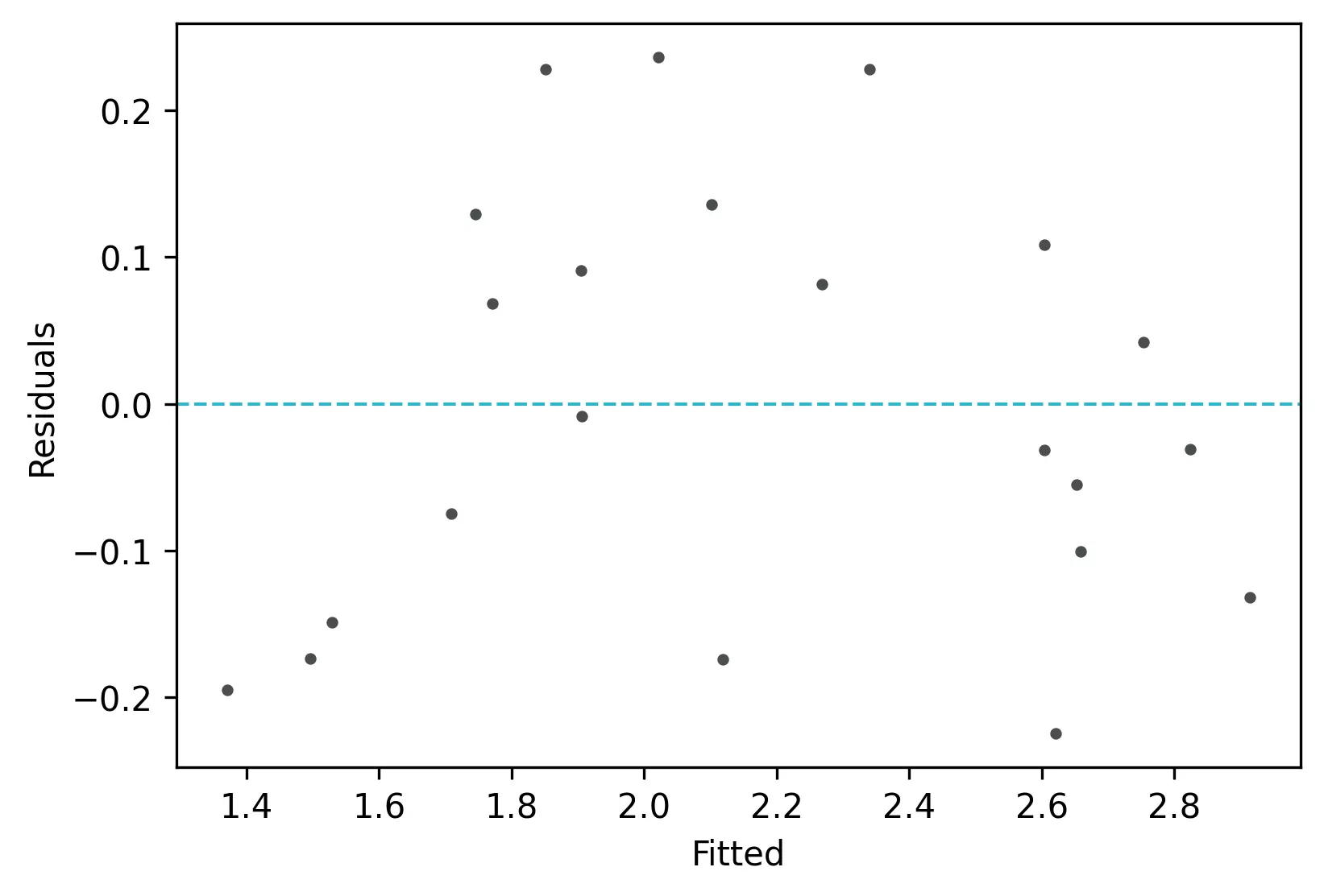
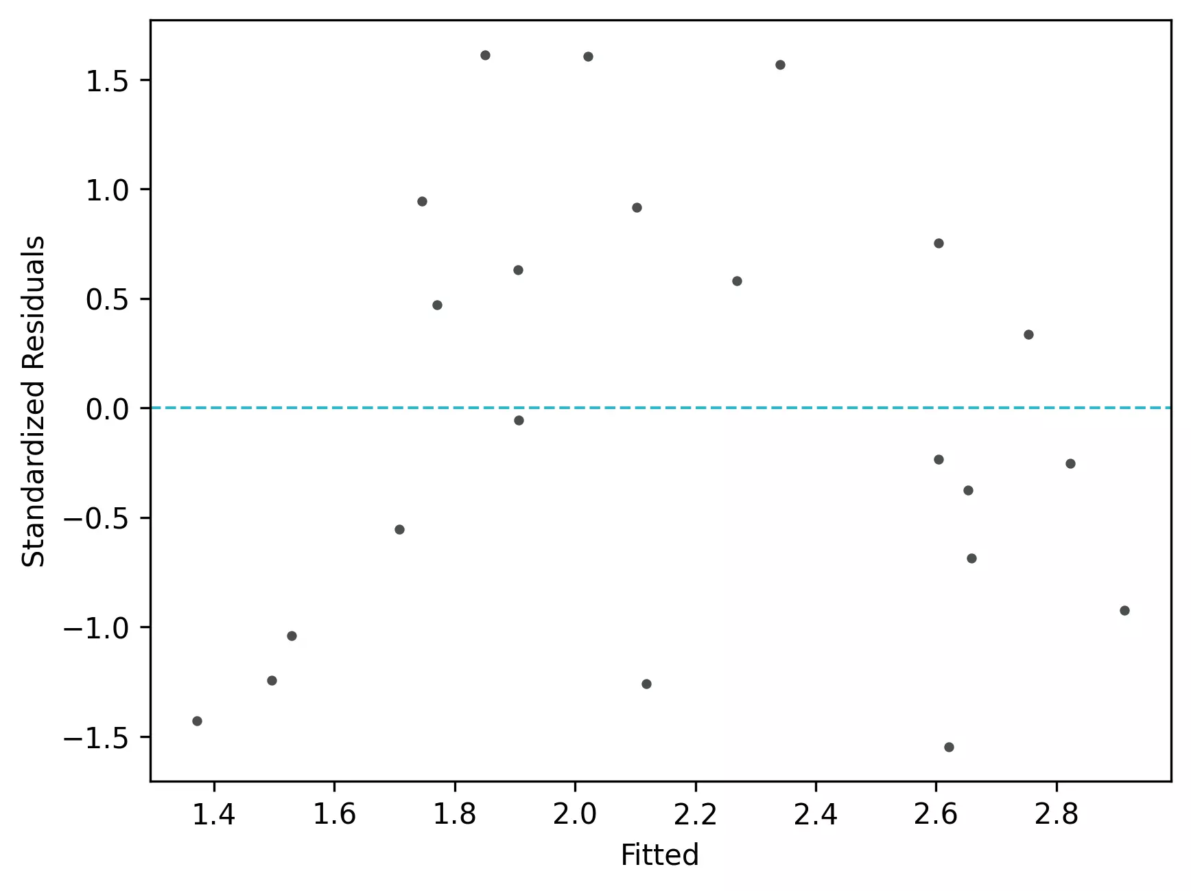
From the plot,
- As the data is pretty equally distributed around the line=0 in the residual plot, it meets the assumption of residual equal variances. The outliers could be detected here if the data lies far away from the line=0.
- In the standardized residual plot, there is no strong visible pattern and data randomly spread around the line. It suggests that it meets assumptions of linearity.
Quantile-quantile (QQ) plot: This plot used to check the data normality assumption
# python
import statsmodels.api as sm
import matplotlib.pyplot as plt

# line=45 option to plot the data around 45 degree line
sm.qqplot(df['std_res'], line='45')
plt.xlabel("Theoretical Quantiles")
plt.ylabel("Standardized Residuals")
plt.show()
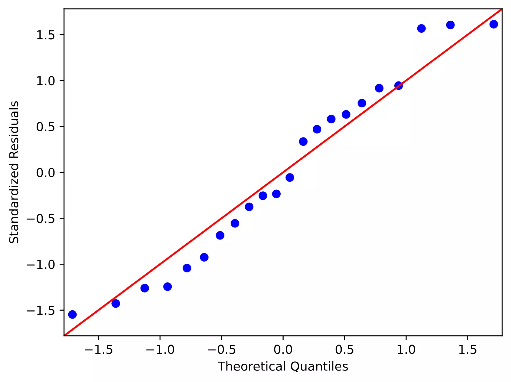
From the plot,
- As the standardized residuals lie around the 45-degree line, it suggests that the residuals are normally distributed
Enhance your skills with courses on regression
- Machine Learning Specialization
- Linear Regression and Modeling
- Machine Learning: Regression
- Machine Learning with Python
Related reading
- Durbin-Watson (DW) test (with R code)
- Multiple linear regression (MLR)
- Mixed ANOVA using Python and R (with examples)
- Repeated Measures ANOVA using Python and R (with examples)
- Multiple hypothesis testing problem in Bioinformatics
References
- Vatcheva KP, Lee M, McCormick JB, Rahbar MH. Multicollinearity in regression analyses conducted in epidemiologic studies.
Epidemiology (Sunnyvale, Calif.). 2016 Apr;6(2). - Ryan TP. Modern regression methods. John Wiley & Sons; 2008 Nov 10.
- McMaster RT. Factors influencing vascular plant diversity on 22 islands off the coast of eastern North America. Journal of Biogeography. 2005 Mar;32(3):475-92.
- https://people.duke.edu/~rnau/rsquared.htm#punchline
- Hoaglin DC. Regressions are commonly misinterpreted. The Stata Journal. 2016 Mar;16(1):5-22.
If you have any questions, comments or recommendations, please email me at reneshbe@gmail.com
This work is licensed under a Creative Commons Attribution 4.0 International License
Some of the links on this page may be affiliate links, which means we may get an affiliate commission on a valid purchase. The retailer will pay the commission at no additional cost to you.